Expand description
§High-order reconstruction and the level set
Not tied to one geometry: the stencil rules and the schemes built on them are checked in one
dimension and, for the finite-volume scheme, in several. Test paths are relative to
crates/merlin-finite-volume/tests/ unless they start with crates/. “Drift” is the relative
change of an integrated quantity between the first and last snapshot.
| Case | Reference | Headline result |
|---|---|---|
| The stencil rules | polynomials, smooth data, a literature table | exact to degree 4 and 10; orders 4.96, 4.98 and 10.65 |
| The reconstruction scheme | exact derivative, exact translation | operator orders 5.1, 5.0 and 10.9; time-integrated 5.00 |
| The stability limits | an independent von Neumann analysis | Courant limits 1.43 (fifth order) and 1.04 (eleventh) |
| A square wave and a bump | exact translation | $L_1$ 4.7e-3 (WENO5), 4.5e-3, 3.7e-3 against MUSCL’s 8.8e-3 |
| The level set | the exact derivative, exact translation, exact time dependence | operator order 5.00 in 1D and 2D (point values), run order 4.9, third order in time |
| Zalesak’s disk and the vortex | the initial shape after a cycle that returns it | Zalesak: 99.2% of the area, 3.1% shape error (WENO5); vortex: order 4.5 to 5.2 |
| PDE reinitialisation | the exact signed distance of a circle | gradient within 4 cells 0.03% at 128 cells, interface unmoved after 500 passes |
| Fast sweeping, and the two compared | the exact signed distance of a circle | whole-grid first-order distance, 1.2% at 128 cells, about 85 times cheaper than the PDE method |
| The Euler equations | the flux Jacobian, exact translation, exact Riemann solution, a fine run | eigenvectors to 1e-14; order 5.0; WENO5 beats MUSCL; primitive is robust, characteristic is accurate |
§The stencil rules
Problem. A rule turns the $2r+1$ cell values around a cell into the value at the cell’s right face.
Weno5 (Jiang and Shu 1996) weights three third-order candidates by their smoothness; LinearUpwind<5> and
LinearUpwind<11> use one fixed combination, the face value of the polynomial through the cells, whose
coefficients are derived from the polynomial-exactness conditions (the derivative of the Lagrange basis of
the primitive function), not tabulated.
Result.
| Rule | Exact up to degree | Order on smooth data (face value of $\sin$) |
|---|---|---|
LinearUpwind<5> | 4 (not 5) | 4.98 |
LinearUpwind<11> | 10 (not 11) | 10.65, rising to 11 as the cells shrink |
Weno5 | linear data exactly | 4.96 |
The five-cell coefficients are $(2, -13, 47, 27, -3)/60$, the table of Shu (1998), reproduced to 1e-14.
Reading it. The exactness tests fail by design for the next degree, so a rule of the wrong order is caught. The eleventh-order rule reaches round-off after a few halvings, so its order is measured on cells up to one radian wide; the pairwise orders climb 10.4, 10.7, 10.8.
Tests that enforce this
Enforced by schemes/stencil_rules.rs: linear_upwind_is_exact_up_to_its_order_minus_one_and_no_further,
the_fifth_order_coefficients_are_those_of_the_literature, the_coefficients_sum_to_one_so_a_constant_is_reproduced,
weno5_weights_are_positive_and_sum_to_one, weno5_on_linear_data_has_the_ideal_weights_and_is_exact,
weno5_is_fifth_order_on_smooth_data, the_linear_rules_have_their_design_order_on_smooth_data,
weno5_stays_inside_the_data_at_a_step_where_the_linear_rule_overshoots.
§The reconstruction scheme
Problem. Reconstruction reconstructs the states on both sides of a face with a rule, in the conserved
variables, and takes the flux from a Riemann flux. For linear advection with the upwind flux the semi-discrete
operator is compared with the exact $-(\sin b - \sin a)/h$ of each cell, and a run of one period with SSP-RK3
is compared with the initial data.
Result. Order of the spatial operator (maximum norm, 32 to 256 cells; 12 to 32 for the eleventh order):
| Rule | Fitted order |
|---|---|
Weno5 | 5.07 |
LinearUpwind<5> | 5.00 |
LinearUpwind<11> | 10.90 |
A run of one period, $L_1$ norm, 20 to 160 cells with the time step falling as $h^{5/3}$ so that the
third-order time error falls as $h^5$ instead of dominating: Weno5 5.00, LinearUpwind<5> 4.99.
A Burgers shock sits at the Rankine-Hugoniot position (0.50000 for WENO5) and WENO5 stays within $10^{-5}$
of the data, where the linear fifth-order scheme overshoots by 0.17. A periodic run conserves the integral to
round-off, and the answer is identical to the last bit for any block layout (1, 2, 3 per axis) and any number of
threads (up to 8), with the eleventh-order rule too, which needs six ghost layers per side; a block narrower
than that is refused with a message naming both numbers.
In more than one dimension the unsplit operator uses the value at the face centre as the face average, which is second order, so the finite-volume scheme is second order there whatever the rule. The rules keep their order in the level set, which works on point values.
Tests that enforce this
Enforced by schemes/reconstruction.rs: the_spatial_operator_has_the_order_of_its_rule,
a_time_integrated_run_is_fifth_order,
a_shock_moves_at_the_rankine_hugoniot_speed_and_only_the_nonlinear_rule_stays_inside_the_data,
a_periodic_run_conserves_the_integral_to_round_off, the_answer_does_not_depend_on_the_blocks_or_the_threads,
threads_alone_do_not_change_the_answer, blocks_narrower_than_the_ghost_layers_are_refused_with_a_clear_error.
A file run reproduces the library-driven run bit for bit (the_high_order_runs_match_the_library_driven_runs_bit_for_bit
in crates/merlin-cli/tests/run/run_from_file.rs).
§The stability limits
Problem. The spectrum of a high-order upwind-biased operator has a large imaginary part. For a Fourier
mode $e^{ik x}$ the semi-discrete eigenvalue is
$z(\theta) = -\big(\sum_j c_j e^{\mathrm{i}(j-r)\theta}\big)(1 - e^{-\mathrm{i}\theta})$ with $\theta = k\,\Delta x$, and one
step multiplies it by the amplification polynomial $R(\nu z)$ of the Runge-Kutta method.
The scheme is stable when $|R(\nu z(\theta))| \le 1$ for all $\theta$.
The scaled eigenvalues $\nu z(\theta)$ of the fifth-order linear operator, against the stability region of SSP-RK3. At the Courant number $\nu=1.43$ the curve fits inside, just short of the limit 1.435; at 1.8 it leaves.
Result.
| Rule | SSP-RK3 | SSP-RK2 | Forward Euler |
|---|---|---|---|
| fifth order | 1.435 | 0.063 | below 0.1 |
| eleventh order | 1.049 | 0.006 | below 0.1 |
The rule reports the SSP-RK3 limit rounded down to 0.01 (1.43 and 1.04; Weno5 takes the fifth-order value), the
solver refuses a larger Courant number with a typed error, and a problem file naming a lower-order integrator is
rejected with the key named. The limits were computed first in an independent Python implementation (1.435 and
1.0493) and the Rust analysis is held to within 0.006 of them.
Tests that enforce this
Enforced by schemes/reconstruction.rs: the_stability_limits_agree_with_an_independent_von_neumann_analysis,
the_solver_refuses_a_courant_number_above_the_limit_of_the_rule, a_shock_is_stable_at_the_advertised_courant_number.
§A square wave and a bump
Problem. The shipped files advection/weno5.toml, advection/upwind5.toml and advection/upwind11.toml
carry a square wave and a smooth bump once around a periodic unit domain at speed 1 (1000 cells, SSP-RK3,
Courant number 0.5, 2000 steps). After one period the exact solution is the initial data.
Result.
| Problem file | $L_1$ error | Min / max of $u$ | Drift |
|---|---|---|---|
advection/weno5.toml | 4.7e-3 | -2.4e-37 / 1.0010 | 1.2e-13 |
advection/upwind5.toml | 4.5e-3 | -0.0607 / 1.0607 | 1.2e-13 |
advection/upwind11.toml | 3.7e-3 | -0.0660 / 1.0660 | 1.2e-13 |
For comparison, the shipped MUSCL file has an error of 8.8e-3 (see the one-dimensional page).
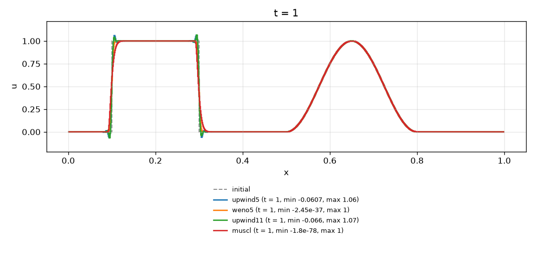
Reading it. All three beat MUSCL on this problem. The linear schemes ring at the jumps (about 6%, a little more at eleventh order), as a fixed stencil must (Godunov’s theorem); WENO5 overshoots by 1e-3 and has no undershoot. Higher order does not remove the ringing of a linear scheme, it narrows it.
Tests that enforce this
Enforced by crates/merlin-cli/tests/run/high_order_problems.rs:
the_high_order_schemes_beat_muscl_on_the_square_wave_and_bump, only_weno5_keeps_the_square_wave_inside_its_range.
§The level set
Problem. The crate merlin-levelset advects a level-set function $\phi$ in a velocity field,
$\phi_t + u\cdot\nabla\phi = 0$ (Osher and Fedkiw 2003). The velocity is a field of its own, a BlockedField with one
component per axis in the blocks of $\phi$, that a source fills at the time of each Runge-Kutta stage (a formula, an
expression of the problem file, and in the multi-material phase the gas); the operator reads it at the cell it updates. The Hamiltonian $u\cdot p$ is linear in the gradient,
so the upwind choice is the sign of $u$: the backward-biased derivative where it is positive, the forward-biased
one where it is negative. Each one-sided derivative is a stencil rule applied to the differences of $\phi$ (Jiang
and Peng 2000), so the three rules and the first-order upwind rule (LinearUpwind<1>) are the ones used for
the flux schemes, with no second copy. The values are point values at the cell centres, not cell averages.
Result. Order of the operator $-u\cdot\nabla\phi$ alone, against the exact derivative of $\sin 2\pi x$ (maximum
norm; 32 to 256 cells, 12 to 32 for the eleventh order, 64 to 512 for the first):
| Rule | Order in 1D | Order in 2D ($\sin 2\pi x \sin 2\pi y$, velocity $(1, 0.6)$, 24 to 64 cells) |
|---|---|---|
| first-order upwind | 1.00 | |
Weno5 | 5.00 | 5.00 |
| Upwind5 | 5.00 | 4.98 |
| Upwind11 | 10.91, rising to 11 |
Unlike the finite-volume schemes, which are second order in more than one dimension because they use the value at the
face centre as the face average, the level set keeps its design order in every dimension: point values need no
transverse quadrature. One period of a translated wave with SSP-RK3 and the time step falling as $h^{5/3}$:
fitted order 0.94 (first order), 4.89 (Weno5) and 4.99 (Upwind5) in 1D, and 4.76 and 4.98 in 2D. With tiny steps on 32
cells, Upwind11 has an error of 2.3e-11 against 1.9e-5 for Upwind5. The operator differentiates a linear function exactly
to round-off for every rule and either sign of the velocity.
Time dependence. A uniform velocity $1 + \tfrac12\sin 2\pi t$ carries a wave through exactly one period, so the exact
solution after time 1 is the initial data. The error falls as the third power of the step, which requires the velocity
to be evaluated at the time of each Runge-Kutta stage (the stage times come from the Shu-Osher form, $c_k = b_k (c_{k-1} + 1)$,
giving 0, 1 and 1/2 for SSP-RK3); a velocity frozen at the start of the step would make the method first order.
Layout. A rotating disk on a 36 by 30 grid gives bit-identical results for one block and for 2 by 3, 3 by 2 and 4 by 1
blocks on one to eight threads, with Weno5 and with Upwind11 (six ghost layers). The solver refuses a field with too few
ghost layers, a Courant number outside the rule’s limit (1.43 for Weno5), a velocity of zero, an integrator of order
below three, a mismatched periodic pair, an end time in the past, and reports a field that has become non-finite. Outflow
ghost cells keep a ramp’s error within 5% of what a wrap-around would give at the ends and many times smaller inside.
The velocity as a field. A named velocity (Uniform, Rotation, ReversingVortex) is sampled into the field at the cell
centres; reading the field gives the same bits as evaluating the formula in every cell, for every rule, block layout and
thread count. The first stage reads the velocity sampled at the end of the previous step (or at time 0), the others are
sampled at their own stage times, and a snapshot holds the velocity of its own time. A named velocity keeps its analytic
bound for the time step. A source with no bound (type = "expression", one expression per axis in x, y, z, or r and z
on a curvilinear domain, and t) is measured instead: the largest $|u_d|$ of the field, taken as a maximum over each block
and then over the blocks (exact in any order, so the same for any number of threads), at the start of every step and at the
stage times of the step before. For a uniform velocity that is the exact bound, and the run is bit for bit the one with the
bound. For a rotation of the unit square it is that of the corner-cell centres, about 1% under the bound of the box. Being a
sample, it can miss a peak between the times sampled or see a growing speed one step late (see the limitations).
A velocity that is not finite is refused at the stage that produces it. The vortex written as an expression
(levelset/vortex_expression.toml, 64 cells) has the velocity of the named vortex to the last bit and a $\phi$ within 1.2e-4
of it, the difference of the two time steps; the rotating circle written as an expression differs by 1.1e-7, and a
three-dimensional constant expression equals the uniform velocity bit for bit. Snapshots hold phi and then the velocity
components u, v, w; the integral reported for a velocity component is not a conserved quantity to check.
From a problem file. [[material]] system = "level_set" gives the interface a velocity
(uniform, rotation about a centre, reversing_vortex, or an expression per axis), the region states give phi, and [numerics] takes
the stencil rule from flux_scheme (first_order for first-order upwind, weno5, upwind5, upwind11) and the
time integrator (third order or more). The run uses the same scheduled driver as the gas, so the snapshot
schedule, the checkpoints and the restart work unchanged. The shipped levelset/translation.toml (a sine wave carried
once round the unit domain) reproduces the library-driven run bit for bit. The shipped levelset/rotating_circle.toml
turns a circle of radius 0.15 once about the centre of the unit square on a 100 by 100 grid:
| Rule | Mean $\lvert\phi-\phi_0\rvert$ inside radius 0.45 | Largest change in the band $\lvert\phi_0\rvert<0.05$ | Area inside the zero level set, start and end |
|---|---|---|---|
| first-order upwind | 1.8e-2 | 6.9e-2 | 0.0716 and 0.0261 |
Weno5 | 3.4e-5 | 6.4e-5 (0.6% of a cell) | 0.0716 and 0.0716 |
| Upwind5 | 4.1e-5 | 4.1e-4 | 0.0716 and 0.0716 |
| Upwind11 | 2.3e-5 | 2.3e-4 | 0.0716 and 0.0716 |
First-order upwind smears away 63% of the circle in one turn; the high-order rules keep the interface within a small fraction of a cell. The error is taken inside radius 0.45 of the centre because the rotation carries values out through the walls beyond radius 0.5, where the outflow ghost cells supply the wrong ones; the orbit of the circle (radius 0.1 to 0.4) never reaches them. A run restarted from a checkpoint on another number of threads ends with the bytes of the uninterrupted run, and the results do not depend on the blocks or the threads.
Tests that enforce this
Enforced by (paths below crates/merlin-levelset/tests/) advection/operator.rs: the_operator_has_the_order_of_its_rule,
in_two_dimensions_the_operator_keeps_its_full_order_unlike_the_finite_volume_schemes,
a_linear_function_is_differentiated_exactly_by_every_rule_for_either_sign_of_the_velocity; advection/translation.rs:
a_translated_wave_has_the_order_of_its_rule_with_the_time_step_refined,
the_eleventh_order_rule_is_far_more_accurate_on_coarse_cells_once_the_time_error_is_small,
in_two_dimensions_a_translated_wave_keeps_the_fifth_order,
a_velocity_that_depends_on_time_is_third_order_in_time_because_each_stage_has_its_own_time; advection/layout.rs:
the_answer_does_not_depend_on_the_block_layout_or_the_thread_count; advection/errors.rs:
a_field_with_too_few_ghost_layers_is_refused, the_courant_number_must_be_positive_and_within_the_limit_of_the_rule,
the_integrator_must_be_of_third_order_or_more, an_outflow_boundary_keeps_a_ramp_much_closer_to_its_exact_motion_than_a_wrap_around;
advection/driver.rs: snapshots_are_written_at_exactly_the_requested_times,
a_run_stopped_at_a_checkpoint_and_restored_continues_with_the_same_bits; advection/velocity.rs:
a_measured_bound_gives_the_bits_of_the_analytic_one_when_they_are_equal,
the_time_step_follows_the_largest_speed_of_the_field_when_it_is_measured,
the_velocity_field_holds_the_velocity_of_the_current_time,
a_peak_between_the_starts_of_two_steps_lowers_the_next_step_when_a_stage_sees_it,
a_velocity_that_cannot_be_produced_at_the_time_of_a_checkpoint_is_reported_as_the_velocity,
a_velocity_that_is_not_finite_is_refused_when_it_is_sampled_and_stops_a_run; and, in
crates/merlin-levelset/src/operator.rs,
reading_the_velocity_from_a_field_gives_the_bits_of_evaluating_it_in_the_operator. The problem files, in
crates/merlin-cli/tests/run/levelset_problems.rs:
a_level_set_file_run_matches_the_library_driven_run_bit_for_bit,
a_circle_comes_back_after_one_turn_with_weno5_and_is_smeared_away_by_first_order,
a_level_set_run_does_not_depend_on_the_blocks_or_the_threads,
a_restarted_level_set_run_ends_exactly_where_the_uninterrupted_run_does,
the_snapshots_hold_the_velocity_the_solver_advected_with,
expression_velocities_agree_with_the_named_types_they_spell_out,
an_expression_velocity_works_in_three_dimensions_and_equals_the_uniform_one; and the configuration, in
crates/merlin-cli/src/config/tests.rs: a_level_set_takes_its_stencil_rule_from_flux_scheme_and_names_its_variable_phi,
a_level_set_refuses_what_is_not_a_level_set_rule_naming_the_key,
the_velocity_of_a_level_set_is_checked_against_the_dimension,
an_expression_velocity_is_checked_for_its_entries_and_its_variables,
a_level_set_writes_its_velocity_with_its_variable.
§Zalesak’s disk and the vortex
Problem. Two standard tests of an interface that is carried and returns to where it started, so that the
initial shape is the exact solution. Both use the unit square, $100\times100$ cells for Zalesak and 32 to 128 for
the vortex, SSP-RK3 and a Courant number of 0.4 and 0.5.
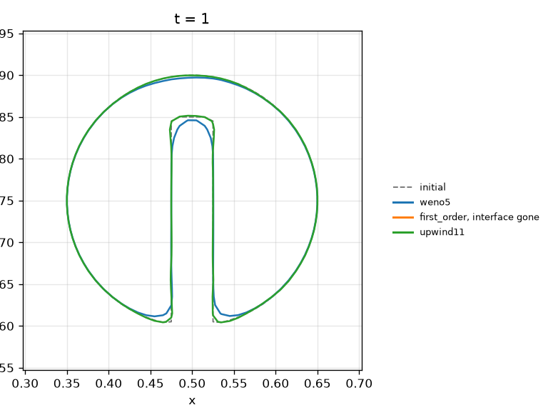
- Zalesak’s slotted disk (Zalesak 1979): a disk of radius 0.15 centred at
$(0.5, 0.75)$, with a slot 0.05 wide and 0.25 long cut up from its bottom edge, turned once about the centre of the square ($\omega = 2\pi$).$\phi=\max(\text{distance to the disk}, -\text{distance to the slot})$, negative inside. It has kinks (the slot corners) but no jumps. The shipped file islevelset/zalesak.toml. - LeVeque’s single vortex (LeVeque 1996): a circle of radius 0.15 at
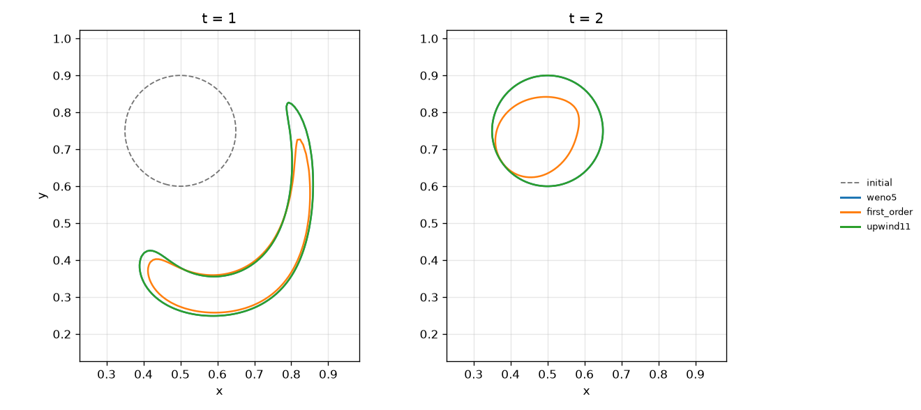
$(0.5, 0.75)$is pulled into a thin spiral by the stream function$\sin^2(\pi x)\sin^2(\pi y)/\pi$, whose flow reverses at half the period, so that at$t=2$the circle returns. The shipped file islevelset/vortex.toml(128 cells).
The two test problems on the unit square. The disk is turned once about the centre; the circle is stretched into a filament by the streamlines of $\psi=\sin^2(\pi x)\sin^2(\pi y)/\pi$ and carried back when the flow reverses at half the period.
Measures. With the smoothed Heaviside function of one cell’s width, $H_\varepsilon(\phi)$ (Osher and Fedkiw
2003, Section 1.4), the area is $\sum (1-H_\varepsilon(\phi))\,\Delta x^2$ and the shape error is the area where
the shape differs from the initial one, $\sum |H_\varepsilon(\phi_0)-H_\varepsilon(\phi)|\,\Delta x^2$, as a
percentage of the initial area. Both shapes are measured the same way, so the smoothing does not bias the difference.
Zalesak, one turn on 100 by 100 cells.
| Rule | Area kept | Shape error |
|---|---|---|
| first-order upwind | 0.56% | 100.3% |
Weno5 | 99.18% | 3.08% |
| Upwind5 | 98.65% | 3.27% |
| Upwind11 | 100.05% | 0.90% |
The vortex, after the flow has reversed. Shape error on 32, 64 and 128 cells, and the observed order between neighbouring grids:
| Rule | 32 cells | 64 cells | 128 cells | Orders |
|---|---|---|---|---|
| first-order upwind | 100% | 99.0% (1% of the area kept) | 46.0% (54% kept) | 0.02, 1.11 |
Weno5 | 9.83% | 0.74% | 0.034% | 3.74, 4.50 |
| Upwind5 | 3.49% | 0.47% | 0.020% | 2.91, 4.57 |
| Upwind11 | 1.48% | 0.13% | 0.0035% | 3.56, 5.19 |
Shape error of the vortex against refinement, each series divided by its own coarsest error.
Reading it.
- First-order upwind cannot carry a thin interface: it keeps 0.6% of Zalesak’s disk and loses the vortex on 64 cells.
- The three high-order rules return the circle after a stretch into a filament a few cells thick with a shape error of
0.03% or less on 128 cells, converging at about the fifth order between 64 and 128 cells (the first pair of grids is
still before the asymptotic range). The order is that of the smooth interface, where the error is that of
$\phi$itself, not of the first order that a discontinuity would limit it to. - On both problems the linear eleventh-order rule is the most accurate and the linear fifth-order rule is no worse than
Weno5. This is because$\phi$has kinks but no jumps, the case a fixed stencil handles well; a function with a jump would make the linear rules ring (see the square wave above).Weno5rounds the closed end of Zalesak’s slot, where the kink is sharpest, and the other rules do not. - The level set is the interface’s position only: nothing here conserves area, and the near-exact areas of the high-order rules are a consequence of their accuracy, not a property of the scheme.
Tests that enforce this
Enforced by crates/merlin-cli/tests/run/levelset_problems.rs:
zalesaks_disk_keeps_its_area_and_its_slot_with_the_high_order_rules,
first_order_upwind_smears_zalesaks_disk_away,
the_vortex_returns_at_fourth_order_or_better_with_weno5,
the_vortex_returns_at_fourth_order_or_better_with_the_linear_fifth_order_rule,
the_vortex_returns_at_fourth_order_or_better_with_the_linear_eleventh_order_rule,
first_order_upwind_loses_the_vortex_even_on_128_cells.
§PDE reinitialisation
Problem. Advection stretches and compresses a level-set function, so $|\nabla\phi|$ drifts away from 1. The
reinitialisation rebuilds a signed distance function with the same zero level set by solving, in pseudo-time,
$\phi_\tau + S(\phi_0)(|\nabla\phi| - 1) = 0$ (Sussman, Smereka and Osher 1994) with the Godunov upwind gradient
(Osher and Fedkiw 2003, Section 7.2) and the WENO5 derivatives of the advection (Jiang and Peng 2000). Three choices
make it work:
- The smoothed sign is
$S = \phi_0/\sqrt{\phi_0^2 + |\nabla\phi_0|^2\Delta x^2}$(Peng et al. 1999), so that a function that is 0.2 or 3 times a distance is treated like one that is a distance. With$\phi_0/\sqrt{\phi_0^2+\Delta x^2}$the 0.2 case had not converged in a band of 8 cells (the gradient was 35% off). - The cells next to the interface are held at their sub-cell distance
$\phi_0/|\nabla\phi_0|$, estimated from central differences (Russo and Smereka 2000), so that the interface does not move. A cell whose slope is already within 5% of one keeps its value (the dead band). Without it, an estimate with an error of its own applied pass after pass moved the interface by 0.11 cells in 10 passes, 0.26 in 100 and nearly a whole cell in 200 (64 cells). - The derivatives are WENO5 whatever rule advects the function: a distance function has kinks where the nearest point of the interface jumps, and the linear eleventh-order rule makes the pseudo-time equation blow up there (the vortex run kept 708% of its area). The reinitialiser works on its own copy of the function, with the three ghost layers WENO5 needs.
Result. A circle of radius 0.25 in the unit square, reinitialised from the exact distance and from 3 and 0.2 times it (a band of 12 cells; the gradient is measured with independent central differences within 4 cells of the interface):
| Cells | Gradient error, distance | 3 times | 0.2 times | Interface position (cells, before and after) |
|---|---|---|---|---|
| 32 | 1.2% | 1.3% | 1.2% | 0.0102 and 0.0102 |
| 64 | 0.17% | 0.29% | 0.19% | 0.0072 and 0.0072 |
| 128 | 0.031% | 0.18% | 0.07% | 0.0026 and 0.0026 |
The interface position is where the function changes sign, found by linear interpolation along the grid lines, so it contains
the error of reading a position that way; reinitialising does not change it. From the exact distance the gradient error falls at
order 2.6. After 500 passes on 64 or 128 cells the position error is the same to four digits and the gradient error has not grown.
A function whose gradient varies by a factor of three ($1 + \tfrac12 \sin 6\pi x \sin 4\pi y$ times the distance) is
restored to 8.5%, 4.0% and 2.35% on 32, 64 and 128 cells, at about first order, because the distance of a cell next to the interface
is estimated from the slope of $\phi_0$ and that slope changes over the cell. A scaled ramp in one dimension becomes the
distance to within 0.006 of a cell. The pseudo-time runs to band cells and the distance function is accurate within about half
of it (two thirds for a wider band): for 3 times a distance on 64 and 128 cells, a band of 8 cells leaves the gradient
1.0% and 1.3% off within 4 cells and 15% and 17% off at 6, where the front that rebuilds it has only just arrived; a
band of 12 cells leaves it 0.3% to 0.8% off within 6 cells and 1.3% to 1.8% off within 8.
In a run. reinitialisation = { method = "pde", every_steps = N, band = 8 } on the level-set material (default
{ method = "none" }) rebuilds the function every N steps; the schedule counts the steps of the run, so a restarted run
continues it. Measured on the shipped problems (a band of 8 cells):
| Problem | Reinitialisation | Area kept | Shape error | $\bigl\lvert\lvert\nabla\phi\rvert-1\bigr\rvert$ near the interface, end |
|---|---|---|---|---|
Zalesak, Weno5, 100 cells | none | 99.18% | 3.08% | |
| every 40 steps | 99.36% | 2.68% | ||
| every 10 steps | 100.37% | 2.33% | ||
Vortex, Weno5, 64 cells | none | 99.40% | 0.74% | 0.117 |
| every 40 steps | 99.18% | 2.02% | 0.022 | |
| every 10 steps | 98.93% | 5.11% | 0.035 | |
| Vortex, Upwind11, 64 cells | none | 100.03% | 0.13% | 0.059 |
| every 40 steps | 100.09% | 3.47% | 0.25 |
Reading it. Reinitialisation does what it is for: it rebuilds a distance function without moving the interface, from any
scale, and as often as asked. It is not free of cost. On the vortex, at its most deformed moment the filament is about two cells
thick, thinner than a distance function can be represented there, and reinitialising then rounds it: the shape error after the
flow has reversed is 3 to 7 times larger than without for Weno5, and 27 to 36 times larger for the linear
eleventh-order rule, whose error without reinitialisation is the smallest of all (0.13%). On Zalesak’s disk, whose features are at least five cells wide, it
slightly improves the corners. So the default is not to reinitialise, and it should be done as seldom as the use of $\phi$
allows (curvature and normals need a distance function; transport alone does not).
Tests that enforce this
Enforced by (paths below crates/merlin-levelset/tests/) advection/reinit.rs:
a_distance_function_is_restored_from_any_scale_and_the_interface_stays_put,
the_gradient_error_of_a_distance_function_falls_at_about_second_order,
a_function_that_is_not_a_multiple_of_a_distance_is_also_restored, reinitialising_many_times_does_not_move_the_interface,
in_one_dimension_a_scaled_ramp_becomes_the_distance_to_its_zero,
reinitialising_does_not_depend_on_the_blocks_or_the_threads,
a_field_with_a_single_ghost_layer_is_reinitialised_in_place_all_the_same, a_reinitialiser_refuses_what_it_cannot_do; and, in
crates/merlin-cli/tests/run/levelset_problems.rs,
reinitialising_the_vortex_restores_a_distance_function_and_costs_the_thin_filament,
reinitialising_zalesaks_disk_keeps_its_area_and_slightly_improves_its_shape,
a_linear_rule_that_advects_can_be_reinitialised_because_the_reinitialisation_uses_weno5; the key of the problem file in
crates/merlin-cli/src/config/tests.rs: a_level_set_is_only_advected_unless_the_file_asks_for_reinitialisation,
the_reinitialisation_of_a_level_set_is_checked_naming_the_key.
§Fast sweeping, and the two compared
Problem. The Eikonal equation $|\nabla\phi| = 1$ can be solved directly, without a pseudo-time, by the fast sweeping
method of Zhao (2005): Gauss-Seidel sweeps over the grid in each of the $2^D$ orderings, each cell taking the
first-order Godunov upwind solution of $\sum_d ((u - a_d)/\Delta x_d)^2 = 1$ from its smaller neighbour along every
axis, until nothing changes (8 sweeps, two rounds of four, for the circle below). The cells next to the interface are held at
the same sub-cell distance as in the pseudo-time method, from one shared estimate (crates/merlin-levelset/src/estimate.rs), so the interface is
placed in the same way. The method is global, because information crosses the grid in one sweep, so it does not split into
blocks: the field is gathered into one array, solved on the calling thread, and written back. It reaches the whole grid
(no band) and has no time step, but it is first-order accurate.
Result. The circle of the previous section, from the exact distance and from 3 and 0.2 times it (the answer is the same for all three, because the held values and the sign are):
| Cells | Gradient error within 4 cells | Within 16 cells | Interface position (cells, before and after) |
|---|---|---|---|
| 32 | 6.9% | 8.1% | 0.0102 and 0.0102 |
| 64 | 2.9% | 7.9% | 0.0072 and 0.0072 |
| 128 | 1.2% | 2.0% | 0.0026 and 0.0026 |
The error falls at order 1.25, as a first-order update gives. A second pass changes nothing, to the last bit (the held cells
are kept by the dead band and the rest is a deterministic function of them), so repeating it cannot drift. A straight line
in one dimension is a distance function and is reproduced to round-off; a scaled sphere on $32^3$ cells has a gradient 9.1%
off within three cells of the surface. The distorted function of the previous section is restored to 10.1%, 4.3% and 2.4% on
32, 64 and 128 cells (against 8.5%, 4.0% and 2.35% for the pseudo-time method): at these values the error is that of the
distance estimated for the cells next to the interface, which the two share. A function of one sign has no interface and is
left as it is, and a NaN is refused with nothing written back.
The two compared, on the circle on 128 cells (a band of 12 cells for the pseudo-time method, one thread each):
| Pseudo-time (WENO5) | Fast sweeping | |
|---|---|---|
| Gradient error within 4 cells, from the exact distance | 0.03% | 1.2% |
| The same, from 3 times the distance | 0.18% | 1.2% |
| Gradient error at 16 cells, from 3 times the distance | 190% (not reached by the band) | 2.0% |
| Time for one reinitialisation (test build) | 144 ms | 1.7 ms |
| A second pass | unchanged to four digits over 500 passes | unchanged to the last bit |
| Order of the gradient error | about 2.6 (exact distance) | 1.25 |
In a run (a reinitialisation every 40 steps, WENO5 advection):
| Problem | None | Pseudo-time | Fast sweeping |
|---|---|---|---|
| Zalesak, 100 cells: shape error, area kept | 3.08%, 99.18% | 2.68%, 99.36% | 5.29%, 97.65% |
| Zalesak, every 10 steps | 2.33%, 100.37% | 6.75%, 96.68% | |
| Vortex, 64 cells: shape error, area kept | 0.74%, 99.40% | 2.02%, 99.18% | 2.50%, 98.54% |
Vortex: $\bigl\lvert\lvert\nabla\phi\rvert-1\bigr\rvert$ at the end, near the interface | 0.117 | 0.022 | 0.061 |
| Vortex, Upwind11 advection: shape error, area kept | 0.13%, 100.03% | 3.47%, 100.09% | 3.39%, 101.31% |
Reading it. Each method wins something, so both are kept. The pseudo-time method is 10 to 40 times more accurate near the interface and slightly improves Zalesak’s corners, but it is confined to its band and about 85 times dearer. Fast sweeping is first-order, so its distance function rounds the corners of the slot (shape error 5 to 7% against 3%) and loses 2 to 3% of the area there, but it costs almost nothing, covers the whole grid, and is exactly idempotent. Use the pseudo-time method where the gradient near the interface matters (normals, curvature) and the features are wide; use fast sweeping where a cheap whole-grid distance is wanted (a signed distance to place things from, or a rough one every few steps). On the vortex’s thin filament both cost accuracy, about equally.
Tests that enforce this
Enforced by (paths below crates/merlin-levelset/tests/) advection/sweeping.rs:
a_distance_function_is_rebuilt_over_the_whole_grid_from_any_scale_and_the_interface_stays_put,
the_gradient_error_falls_at_about_first_order,
a_function_that_is_not_a_multiple_of_a_distance_is_restored_as_well_as_by_the_pseudo_time_method,
a_second_pass_changes_nothing_at_all, in_one_dimension_a_scaled_ramp_becomes_the_distance_exactly,
in_three_dimensions_a_scaled_sphere_becomes_a_distance_function,
a_function_with_one_sign_has_no_interface_and_is_left_alone, a_field_with_a_nan_is_refused_and_left_alone,
compared_with_the_pseudo_time_method_it_is_less_accurate_near_the_interface_but_covers_the_grid; and, in
crates/merlin-cli/tests/run/levelset_problems.rs,
fast_sweeping_rebuilds_the_distance_function_of_the_vortex_over_the_whole_grid,
fast_sweeping_is_less_kind_to_zalesaks_corners_than_the_pseudo_time_method.
§The Euler equations
Problem. The reconstruction works in one of three sets of variables. The conserved ones are the
unknowns themselves. The primitive ones are density, velocity and pressure (Equation::to_primitive).
The characteristic ones are $w = L u$, with $L$ the left eigenvectors of the flux Jacobian at the face
(Equation::left_eigenvectors, built from Toro 2009, Section 3.2), so that each component is one wave;
the eigenvectors are evaluated at the mean of the two conserved states next to the face. A state a
reconstruction makes unphysical (negative density or pressure) is replaced by the cell value.
Four things are compared with a reference: the eigenvectors with the flux Jacobian; a smooth density wave
carried once round a periodic unit domain (the exact solution is the initial data); Toro’s five shock tubes
with the exact Riemann solution ($L_1$ error of the density as a fraction of its range, 400 cells, HLLC,
SSP-RK3, Courant number 0.4 unless stated); and Shu and Osher’s problem (1989, Example 8), a Mach 3 shock
running into a sinusoidal density on $[-5, 5]$ to time 1.8, with a fine run of the same code.
The eigenvectors. For one, two and three velocity components, over 200 random states and two values of
$\gamma$, $L R$ equals the identity to 1e-14, and $R\,\mathrm{diag}(\lambda)\,L$ equals the flux
Jacobian, computed independently by central differences, to 3e-10 (the error of the differences). Swapping two
columns, or two eigenvalues, is caught at 1e-2 or more.
Smooth wave. On 20 to 160 cells, the time step falling as $h^{5/3}$, the fitted order is 4.98 to 5.01 for
Weno5 and for the fifth-order linear rule in all three sets of variables.
Toro’s tests.
| Problem | MUSCL | Weno5 conserved | Weno5 primitive | Weno5 characteristic | Linear 5, 11 |
|---|---|---|---|---|---|
| 1 (Sod) | 0.0017 | 0.0015 | 0.0013 | 0.0015 | 0.0017 and 0.0024 (0.0012 and 0.0023 primitive) |
| 2 (123, towards vacuum) | 0.0024 | 0.0031 | 0.0020 | blows up, at every Courant number from 0.4 to 0.02 | blow up |
| 3 (pressure ratio 1e5) | 0.0077 | 0.0056 | 0.0057 | 0.0053 | blow up |
| 4 (colliding shocks) | 0.0052 | 0.0046 | 0.0043 | 0.0046 | blow up |
| 5 (1e5, flow of speed 19.6) | 0.0019 | blows up at every Courant number from 0.4 to 0.01 | 0.0031 at 0.3 and below, blows up at 0.4 | 0.0013 at 0.15 and below, blows up at 0.2 and above | blow up |
On Sod’s tube Weno5 converges at order 0.9 in every choice of variables from 100 to 800 cells, first order as
expected for a problem with a contact; the first-order scheme has 0.0102 at 400 cells.
Shu and Osher’s problem. Error of the density against the reference, as a fraction of its range:
| Cells | MUSCL | Weno5 conserved | Weno5 primitive | Weno5 characteristic | Upwind5 | Upwind11 |
|---|---|---|---|---|---|---|
| 200 | 0.0201 | 0.0188 | 0.0186 | 0.0165 | 0.0105 | 0.0086 |
| 400 | 0.0153 | 0.0068 | 0.0068 | 0.0054 | 0.0031 | 0.0032 |
| 800 | 0.0069 | 0.0029 | 0.0030 | 0.0022 | 0.0013 | 0.0016 |
The reference is Weno5 in the characteristic variables with HLLC on 8000 cells (Courant number 0.3),
averaged onto 1600 cells and stored in tests/data/shu_osher_reference.csv; the example
shu_osher_reference regenerates it. It comes from the code it is used to test, so this measures how a
coarser run approaches a much finer one, not that the answer is right. The shipped euler/shu_osher.toml
(400 cells, characteristic) has the error 0.0054, and the same file with MUSCL 0.0153.
Cost. Speed of the shipped Shu and Osher problem on 4000 cells, one thread, release build, median of five alternating runs (the spread within each variant is 3% or less):
| Variant | Million cell updates per second | Relative to Weno5 conserved |
|---|---|---|
| MUSCL, van Leer | 10.4 | 1.87 |
Weno5 conserved | 5.57 | 1.00 |
Weno5 primitive | 4.90 | 0.88 |
Weno5 characteristic | 3.14 | 0.56 |
| Upwind5 | 7.19 | 1.29 |
| Upwind11 | 6.18 | 1.11 |
| Upwind11 characteristic | 3.65 | 0.59 |
The characteristic variables cost about 1.8 times the time of the conserved ones, for the eigenvector products at each
face. As a rough equal-cost comparison from the two finest grids above (conserved Weno5 improves 2.3 times from 400 to
800 cells, order about 1.2): matching the characteristic error at 400 cells (0.0054 against 0.0068) takes about 1.2
times the cells and 1.4 times the work, which at these speeds is about 20% cheaper than the characteristic variables.
On Shu and Osher’s problem the accuracy they gain therefore does not pay for their cost; their case is Toro’s fifth
test, where they are the most accurate choice that survives.
Reading it.
Weno5is more accurate than MUSCL on four of the five of Toro’s problems and on Shu and Osher’s, without a positivity limiter.- Primitive variables are the robust choice. They survive tests 1 to 4 and test 5 at a Courant number of 0.3 or less.
- Characteristic variables are the accurate choice. They are 12% (200 cells) to 24% (800 cells) better than the
others on Shu and Osher’s problem and 2.4 times better than the primitive ones on test 5, but they fail on the vacuum-like
test 2, where
$1/c$in the eigenvectors is badly conditioned, and need a Courant number of 0.15 or less on test 5. - The conserved variables win no case. For
Weno5they are never the most accurate on any problem above (6% to 55% worse than the best choice), and the only choice that cannot pass test 5. They are kept as the default because they are the cheapest and because for the linear rules they are equal to the characteristic variables (next point); whether to keep them as a choice forWeno5is an open decision (the roadmap, 8.3, drops a variant that wins on no case). - For a linear rule the characteristic variables give the conserved result (the flux differs by 4e-16): the reconstruction is linear, the eigenvectors are the same across the window, and a linear operation commutes with a fixed matrix. The choice only matters for the nonlinear rule.
- The linear rules are the most accurate on Shu and Osher’s problem, about twice as accurate as
Weno5in this range of grids, because the shock is weak and the rest is smooth. They are not positivity preserving: on every strong problem their oscillations take the pressure negative and the run ends with a non-finite solution, in any variables, even though a state that is unphysical at a face is replaced by the cell value (the cell itself is updated unphysically). A positivity-preserving limiter (Zhang and Shu 2010) would be the remedy and is not part of this phase. - The answer does not depend on the block layout (1, 4 or 6 blocks) to the last bit.
Tests that enforce this
Enforced by crates/merlin-systems/tests/equations/eigenvectors.rs: the_gas_eigenvectors_invert_each_other_and_diagonalise_the_flux_jacobian,
a_wrong_set_of_eigenvectors_is_caught_by_the_same_check, the_acoustic_eigenvectors_of_a_gas_at_rest_are_the_textbook_ones,
a_scalar_law_has_the_single_eigenvector_one; equations/euler_high_order.rs:
a_smooth_density_wave_is_fifth_order_in_every_choice_of_variables,
every_rule_in_every_choice_of_variables_captures_sods_tube_far_better_than_first_order,
weno5_converges_on_sods_tube_at_about_first_order, weno5_keeps_the_strong_problems_that_the_linear_rules_cannot,
the_characteristic_variables_carry_weno5_through_tests_three_and_four_but_not_two,
on_the_fifth_problem_only_the_primitive_and_characteristic_variables_survive_and_the_latter_is_more_accurate,
for_a_linear_rule_the_characteristic_variables_give_the_conserved_flux_and_for_weno5_they_do_not,
on_the_shu_osher_problem_the_high_order_schemes_beat_muscl_and_weno5_does_best_in_the_characteristic_variables,
the_shu_osher_error_falls_as_the_grid_is_refined, the_answer_does_not_depend_on_the_number_of_blocks;
schemes/reconstruction.rs: for_a_scalar_law_the_primitive_variables_are_the_conserved_ones. The shipped
euler/sod_weno5.toml has the published plateau values (sods_weno5_problem_has_the_published_plateau_values) and
reproduces the library-driven run bit for bit (a_weno5_file_run_matches_the_library_driven_run_bit_for_bit), and
euler/shu_osher.toml is close to the reference (the_shu_osher_file_run_is_close_to_the_reference_and_muscl_is_not),
all in crates/merlin-cli/tests/run/euler_problems.rs.