Module limitations 

Known limitations

This page lists where the schemes are expected to fail, with the runs that show it, and what the validation does not cover. The failures are demonstrations, not bugs: each has a counterpart in the validation pages that does the same thing correctly. Problem files are in problems/.

Where schemes are expected to fail

First-order smearing, and the cost of second order without a limiter

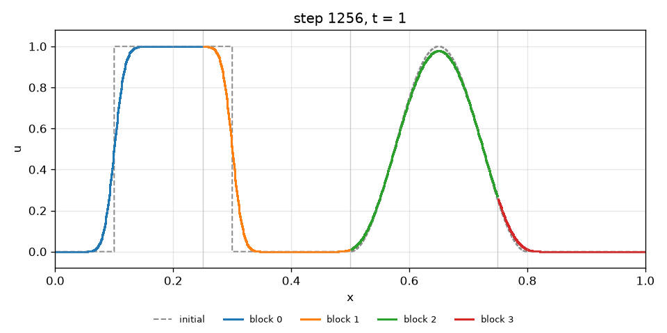
First-order upwind advection (1d/advection/upwind.toml) pays for monotonicity with numerical diffusion: the square wave becomes a rounded step and the bump loses its peak. Its $L_1$ error after one period is 2.67e-2, three times MUSCL’s 8.82e-3, and its order is 1.

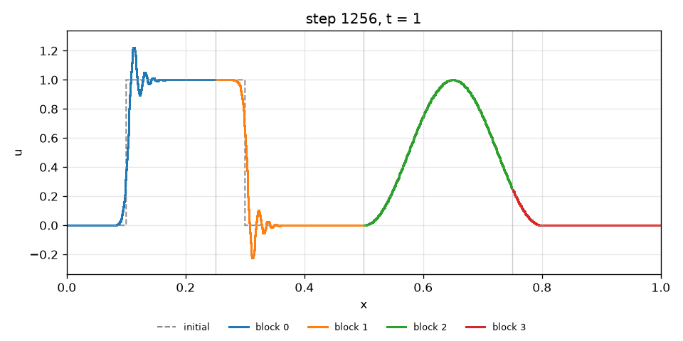
Lax-Wendroff is sharper but, being a linear second-order scheme, it cannot also be monotone (Godunov’s theorem): it overshoots to 1.222 and undershoots to -0.222 at the two jumps. The limited MUSCL scheme keeps the solution inside $[0,1]$.

The Roe flux without an entropy fix

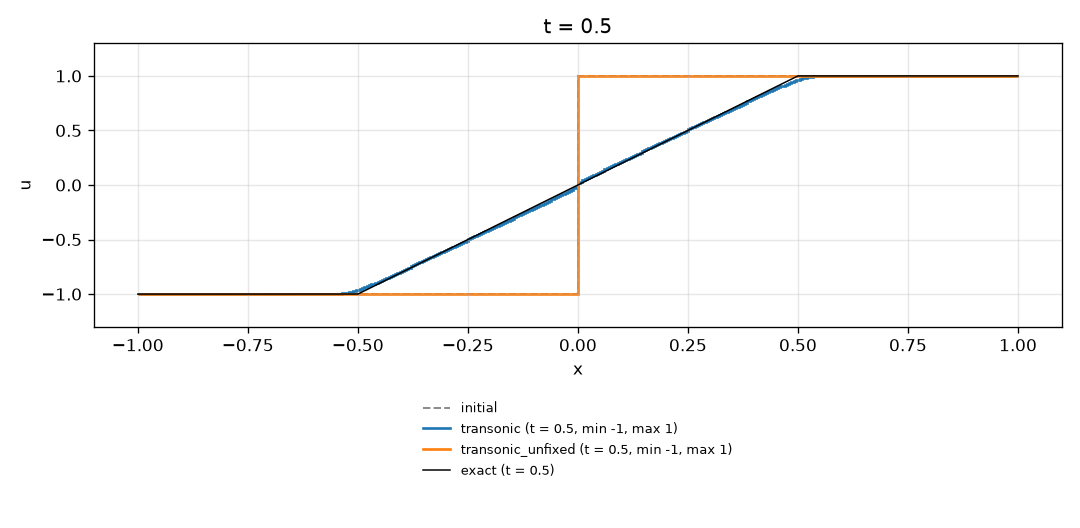
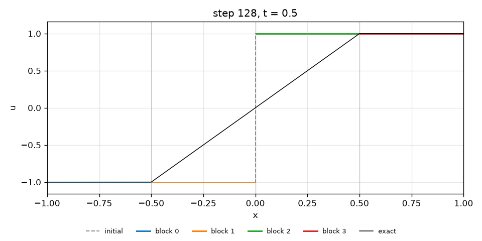
1d/burgers/transonic_unfixed.toml runs the transonic problem with riemann_solver = "roe_no_fix". At the sonic point the Roe speed is zero, so the jump never moves: it stays a stationary discontinuity from -1 to +1, an expansion shock that violates the entropy condition and is not the solution of Burgers’ equation (Roe 1986; LeVeque 2002, §12.3, on the Harten-Hyman fix).

Flux	$L_1$ error at $t=0.5$	$L_\infty$ error	Two cells at $x=0$
Godunov (entropy-satisfying)	1.32e-2	0.036	-0.019, +0.019
Roe, no entropy fix	0.500	0.995	-1, +1

The integral does not change in either run (zero by symmetry), so conservation does not reveal the failure; only the comparison with the exact solution does. Away from sonic points the two fluxes agree.

HLL smearing a contact

The stationary contact of the 1D page again, with riemann_solver = "hll" in a copy of the file. HLL has two waves and no contact wave, so it diffuses the contact; HLLC and the exact flux do not.

Flux	$L_1$ density error	Max density error	Cells strictly between the two states	10 to 90 % width
HLLC	0	0	0	0 cells
HLL	6.17e-3	0.399	43	9 cells

Velocity and pressure stay exactly uniform in both runs, and mass and energy are unchanged.

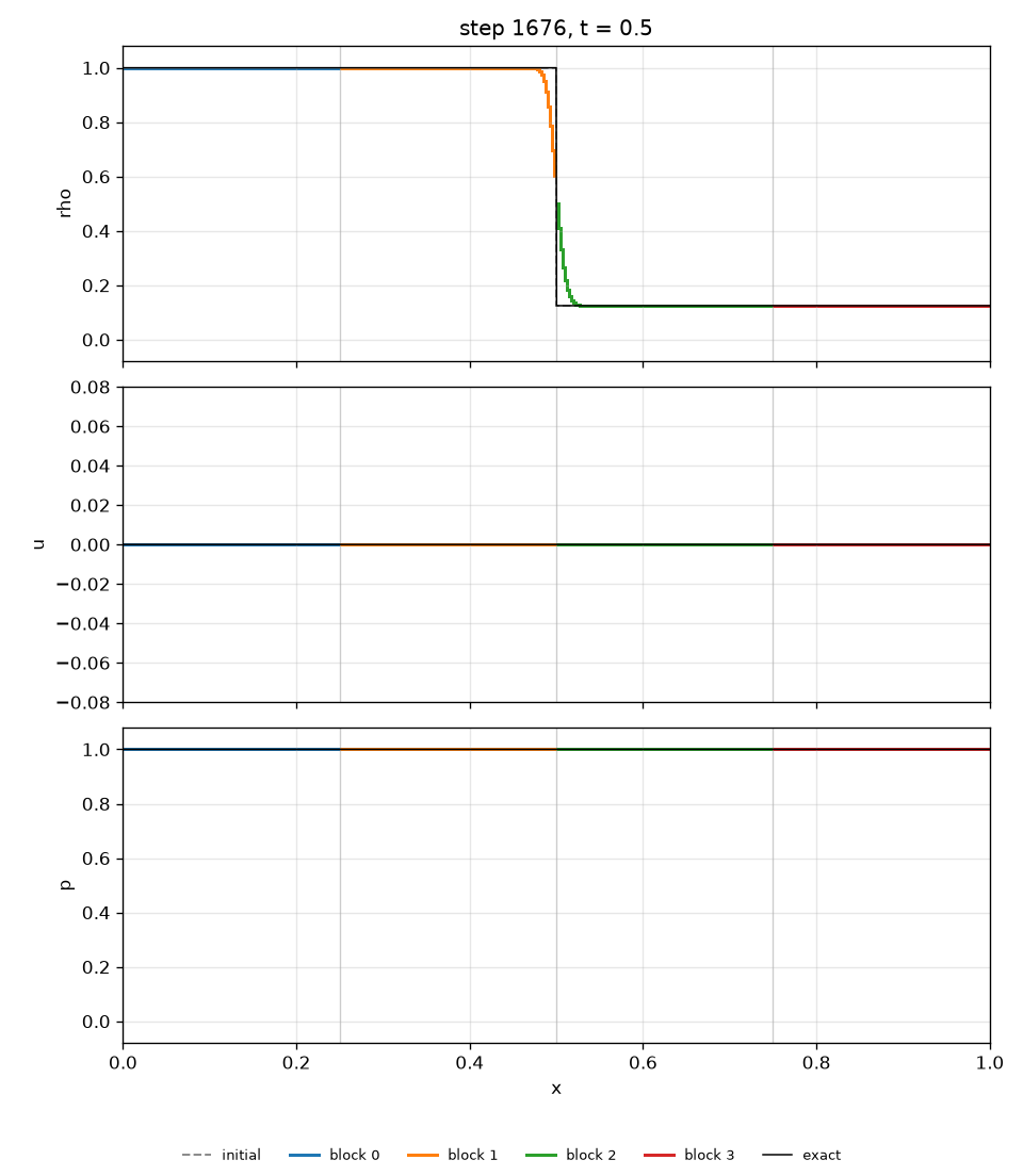
For Sod’s problem the difference is small, because MUSCL already sharpens the contact: $L_1$ density error 1.65e-3 with HLLC against 1.73e-3 with HLL.

Hard cases converge slowly

• The near-vacuum centre of Toro’s test 2: the central pressure is 0.00335 against 0.00189 on 400 cells.
• Contacts are smeared over several cells in the strong tests (7 cells, 10 to 90 %, in the colliding-shock problem).
• A 2 % overshoot at the foot of the blast fan and ripples of about 0.5 % on the colliding-shock plateau.
• Noh’s implosion shows the wall-heating error at the centre in both geometries.

Reinitialisation of the level set

• Both methods cost accuracy somewhere, so neither is on by default. The pseudo-time method is confined to its band and, on features thinner than the band (the vortex filament), it makes the shape error worse (0.74% to 2.0% on 64 cells). Fast sweeping is first order and global: it rounds the corners of Zalesak’s slot (shape error 5.3% every 40 steps, 6.8% every 10, against 3.1% without). Fast marching is not implemented. See the comparison.
• Fast sweeping gathers the whole grid and runs on one thread. It copies the level set into one array and sweeps it serially, the one piece of the level-set code that is not block-local, so it does not speed up with the number of threads and could not run on a distributed grid. The pseudo-time method is block-local and runs on all threads.
• An expression velocity has a measured time-step bound. A formula given as type = "expression" has no known bound on its speed, so the solver takes the largest $|u_d|$ of the sampled field at the start of each step and at the stage times of the step before, and the next time step from the largest of them. That is a sample at the cell centres and at those times: a speed that peaks between them, or that grows during the step it is first seen in, is missed or seen one step late, and a velocity that changes quickly in time needs a smaller Courant number. The named velocities (uniform, rotation, reversing_vortex) have exact bounds, so their time step does not change.
• The finite-volume high-order schemes are second order in 2D and 3D. The unsplit operator uses face-midpoint fluxes, so WENO5 and the linear rules show their design order only in 1D; the level set keeps it in any dimension. The reconstruction schemes are refused on cylindrical and spherical grids.
• The linear rules (Upwind5, Upwind11) oscillate at shocks by design, and need a third-order or better time integrator and a Courant number within the limit of the rule (1.43 and 1.04).

What is not covered

• Curvilinear geometry is for the gas. Cylindrical and spherical coordinates run the Euler equations. Swirl (azimuthal velocity) is available on a cylindrical domain only; a spherical domain has no swirl or tangential velocity, and there is no spherical 2D or 3D (only a radius). Lax-Wendroff is refused in both. The output files call the axes x, y, z whatever the geometry (the plots label them r and z, reading the geometry from the problem file), so for these runs x is the radius.

• The time step costs more near the axis. The radial speed of the cell next to the axis is multiplied by its face area over volume (2 for a cylinder, 3 for a sphere), so steps are up to 2 to 3 times shorter when the fastest wave is in that cell. This keeps the Courant number of every cell at most the nominal one and a strong outward flow at the axis positive; the price is paid for every run in these geometries.

• The angular momentum is reported, not the swirl momentum. The plain integral of $\rho w$ is not constant, so the output reports $\int r\rho w\,dV$ as angular_momentum. Its conservation is exact (a drift of 0 in the cases of the cylindrical page); the swirl is validated against an exact steady state and the invariants, but there is no unsteady swirl solution to compare with.

• Sedov’s solution is a bound, not an order. The reference is the point-source limit and the runs start from a ball of finite size, so the error stops falling at a few parts in a thousand. The Sedov and cylindrical sound-wave checks run from Python in continuous integration, not in cargo test; the Rust test of the same radial source terms is the spherical sound wave.

• One material per run. An ideal gas, a stiffened gas (the water tube) or a Mie-Gruneisen solid (the copper impact), with one law per run. A solid is a fluid here: no strength, no shear, no tension limit. A fluid other than the ideal gas offers only the hllc flux from a problem file and no exact flux: the exact flux is written for the ideal gas only until it is rebuilt on the matching solve, and the others are in the library (and its tests) and not in the problem files. A flux no longer adds copies of the solver to the program (the scheme is chosen at run time in the materials build, phase 9.1c). The shock-bubble uses a lighter bubble of the same gas, not the helium bubble of the experiments.

• The scalar laws are a build of their own. Advection (with Lax-Wendroff) and Burgers’ equation are in the cargo feature scalar of merlin-cli, not in the default build, which holds the fluids and the level set. In the scalar build Lax-Wendroff is about 11 % slower at one thread than before the split (4.71 s against 4.23 s on the 2D case of scripts/timing-cases.py); advection and Burgers are unchanged. The cause was not investigated.

• The scheme is a run-time choice in the materials build, so each face costs a call through a table. The cheapest scheme (MUSCL with HLL, on 512 by 512 and 1024 by 1024 cells) is 7 to 9 % slower at one thread than when every scheme was compiled in; the other gas cases are as fast or faster. The small functions below the scheme are forced inline, and a new Riemann solver or equation needs the same care (.claude/rules/kernels.md).

• Several materials run from code only, and with no physics at the interface yet. The coupled solver (coupled materials) is in the library and in an example; there is no problem-file syntax for it before phase 9.3. The ghost cells of a material hold the extension of its own real state along the normal, which is first order in the position of the interface and has no pressure or velocity matched across it: a shock that reaches an interface is not transmitted to the other material. So it moves interfaces and keeps a state for each material on both sides; it does not yet model a shock crossing a material interface (9.3 and 9.4).

• The mass of a material over its real cells is not conserved at an interface. It changes as the number of cells it owns does, as the interface crosses the grid: in a bubble in uniform flow, by +0.20 % (ambient) and -1.21 % (bubble) at 48 by 48 cells and $t=0.2$, and by -0.009 % and +0.058 % at 128 by 128 and $t=1$. Measured and reported, not corrected.

• A coupled step is expensive and the level-set functions are not reinitialised. Two materials cost 3.80 times a one-gas step at one thread and 5.95 times at eight (256 by 256 cells, MUSCL with HLL), against 2 for the operators alone; the sweeps over the whole grid for a thin band are the suspects, and nothing was profiled. A second way of filling the ghost cells (fast marching) and the reinitialisation of the functions in a coupled run are not built either. All three are the roadmap entry 9.2b, to be done before the long runs of 9.4.

• The level-set solver is compiled for every dimension and stencil rule. The materials build holds 12 copies of the level-set operator and solver (3 dimensions times the 4 rules first_order, weno5, upwind5 and upwind11) and 3 of the reinitialisation, because the rule is a generic parameter that the operator calls for every cell. Unlike the flux scheme (chosen at run time since phase 9.1c) it is not boxed, on purpose: in phase 9.2 a spike that chose the rule at run time (the rule read through a window of its values and one call through a table, one instance per dimension; output bit-identical) was measured on levelset_zalesak (400 by 400 cells, 1571 steps) and levelset_vortex (512 by 512, 1024 steps) of scripts/timing-cases.py, WENO5 with SSP-RK3, median of three runs on an Apple M1:

  Case	Threads	Rule compiled in	Rule at run time	Change
  Zalesak	1	16.70 s	20.43 s	+22.3 %
  Zalesak	8	5.43 s	6.61 s	+21.7 %
  Vortex	1	31.70 s	36.77 s	+16.0 %
  Vortex	8	8.65 s	9.68 s	+11.9 %

  and the clean release build of merlin-cli (one run each) went from 40 s to 37 s (-7.5 %), from 869 MB to 831 MB of compiler memory (-4.4 %) and from 3,930,424 to 3,788,488 bytes (-3.6 %), with the copies of HjOperator::apply falling from 24 to 6. The level set slowed by 12 to 22 % for a saving of 3 s and 38 MB, so it stays generic. The copies are not multiplied by the number of materials in the coupled solver, which uses one operator for every level-set function. The record is in the Outcome of docs/plans/phase-9.2-coupled-solver.md.

• Burgers’ equation runs from a file in 1D only, although the library supports more. A fixed-state inflow boundary is available in the library but not from a problem file for a gas; use outflow.

• The 2D Riemann problems have no exact solution. Only derivable features are asserted (symmetry, conservation, positivity, jump conditions, refinement), and the final times and the discontinuity position of configuration 3 are chosen, not taken from the paper.

• No order of convergence is measured on the shock problems themselves beyond what the test suite does; order is measured on smooth data (the 1D density wave, the 2D vortex, the sound waves, solid-body rotation), and plateau values and positions on the shock problems (Noh and Sedov included).

• Resolution. The figures use one resolution (400 cells for the shock tubes, 100 to 400 per side in 2D).

• Speed. Parallel speedup is limited by memory bandwidth (2.55 times on 4 threads of an M1 for the 100 by 100 vortex). Timings are one machine on one day, and no test asserts a speedup.

• XDMF. The scalar files were opened in VisIt by hand and the tests confirm that every reference resolves with the declared shape. The velocity is also written as a vector attribute (components u_x, u_y, u_z in Cartesian space, u_r, u_z, u_θ in cylindrical, labels stored with the data), but VisIt has not been checked on it, in particular on a two-component vector in 2D. The HDF5 file stays locked while a run writes it.

References

• Roe, P. L. (1986), Characteristic-based schemes for the Euler equations, Annu. Rev. Fluid Mech. 18.
• LeVeque, R. J. (2002), Finite Volume Methods for Hyperbolic Problems, Cambridge.
• Godunov, S. K. (1959), A difference scheme for numerical solution of discontinuous solution of hydrodynamic equations, Mat. Sbornik 47 (the theorem that a monotone linear scheme is first order).